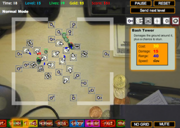
I made a "tool" with google sheets to compare costs and damage between up to three towers. (May I add it as a resource?)

Link: https://docs.google.com/spreadsheets/d/1uOzjkzzey0hH2PYF_rmo4R15HgsBYUjj8jcb-YpI2ys/edit?usp=sharing

Info: It automatically compares two sets of towers (max. 3 different towers, you can multiply xX amount). It can help you decide whether or not to replace a set of towers with another or help you find new ideas.

How to use:

1. Make a copy of the file in google sheets if you can't edit (File - Make a Copy...)
2. There's a light gray box and a dark gray box
   • Light gray is for calculating tower costs and damage
   • Gray is for comparing two sets of towers (only output)
3. Edit ONLY the ORANGE, GREEN, and YELLOW cells (inputs)
4. The possible inputs are INSIDE the RED BORDERS.
5. The outputs will change automatically. Do not edit the output cells.

Example: I have a LVL2 Swarm Tower and I want to know if it's better to upgrade it to LVL3 or place another LVL1 Swarm Tower

Input: Set 1: One Swarm Tower LVL1+One Swarm Tower LVL2 Set 2: One Swarm Tower LVL3

Output: Set 1 Cost:130 Damage:60 Cost/Damage: 2.166666667

Set 2 Cost130 Damage: 80 Cost/Damage: 1.625

It seems that Set 2 (One Swarm Tower LVL3) is better since it does more damage at the same cost. But it depends on what you want: more range of attack and attack speed (Option 1) or more damage in a small area (Option 2).

I will be updating, any advice is welcome.

I love spreadsheets so much, I started doing them at the end of middle school, throughout all of high school for whatever reason I could find, and now I make spreadsheets for my day job, check out the cool formula I made today, pretty simple, but convoluted enough to where it looks cool

=IF(IF(AH90="",AG90&" ("&VLOOKUP(O90,$A$1:$F$15,6,FALSE)&")",IFERROR(IF(AND(VLOOKUP(O90,$C$23:$D$36,2,FALSE)=VLOOKUP(P90,$C$23:$D$36,2,FALSE),AI90=""),AG90&" ("&VLOOKUP(O90,$A$1:$F$15,6,FALSE)&", "&VLOOKUP(P90,$A$1:$F$15,6,FALSE)&")",IFERROR(IF(AND(VLOOKUP(O90,$C$23:$D$36,2,FALSE)=VLOOKUP(P90,$C$23:$D$36,2,FALSE),AJ90=""),AG90&" ("&VLOOKUP(O90,$A$1:$F$15,6,FALSE)&", "&VLOOKUP(P90,$A$1:$F$15,6,FALSE)&", "&VLOOKUP(Q90,$A$1:$F$15,6,FALSE)&")"),"")),""))=FALSE,AG90&" ("&VLOOKUP(O90,$A$1:$F$15,6,FALSE)&", "&VLOOKUP(P90,$A$1:$F$15,6,FALSE)&", "&VLOOKUP(Q90,$A$1:$F$15,6,FALSE)&", "&VLOOKUP(R90,$A$1:$F$15,6,FALSE)&")", "")

then all of those cells go through a bunch of index match formulas =IFERROR(INDEX($A$1:$E$15,MATCH(R90,$A$1:$A$15,0),MATCH($N90,$A$1:$E$1,0)), "")

Thank you for sharing. I would like to know how does your formula work. I see that some cell references refer to row number 90 and others like $C$23:$D$36 and $A$1:$F$15. What is it supposed to be there?

those are just the arrays that are being looked at, they're just charts of information